Dimensional queries are designed to enable multiple-fact querying. The basic goals of multiple-fact querying are:
Preserve data when fact data does not perfectly align across common dimensions, such as when some fact data is missing for certain dimensional values but other facts are present.
Prevent double-counting when fact data exists at different levels of granularity by ensuring that each fact is represented in a single query with appropriate grouping. Determinants may need to be created for the underlying query subjects in some cases.
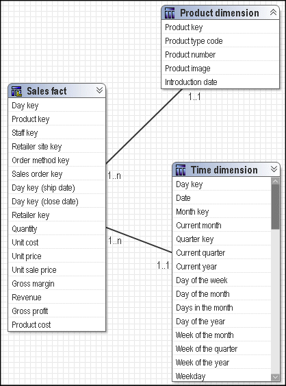
A query on a star schema group results in a single fact query.
In this example, the Sales fact is the focus of any query that is written. The dimensional query subjects provide attributes and descriptions to make the data in Sales fact more meaningful. All relationships between dimensions and the fact are 1-n.

When you filter on the month and product, the result is as follows.
| Month | Product | Quantity |
| January | TrailChef Water Bag | 62,791 |
| January | TrailChef Canteen | 27,229 |
| January | TrailChef Kitchen Kit | 20,785 |
| January | TrailChef Cup | 29,670 |
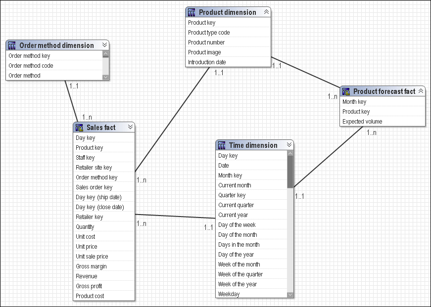
A query on multiple facts and conformed dimensions respects the cardinality between each fact table and its dimensions and writes SQL to return all the rows from each fact table.
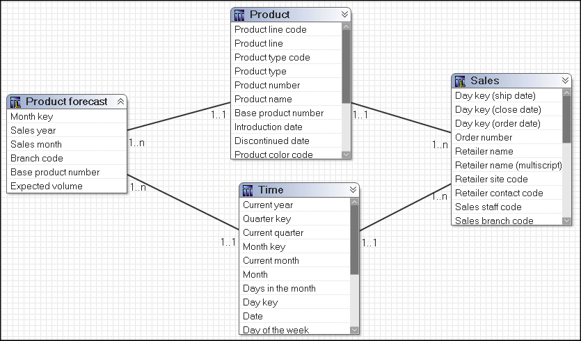
For example, Sales and Product forecast are both facts.

Note that this is a simplified representation and not an example of how this would appear in a model built using Cognos modeling recommendations.
Individual queries on Sales and Product forecast by Month and Product yield the following results. The data in Sales is actually stored at the day level.
| Month | Product | Sales target |
| Opening balance | ||
| January | TrailChef Water Bag | 4,053,900 |
| January | TrailChef Canteen | 4,053,900 |
| January | TrailChef Kitchen Kit | 4,053,900 |
| January | TrailChef Cup | 4,053,900 |
A query on Sales and Product forecast respects the cardinality between each fact table and its dimensions and writes SQL to return all the rows from each fact table. The fact tables are matched on their common keys, month and product, and, where possible, are aggregated to the lowest common level of granularity. In this case, days are rolled up to months. Nulls are often returned for this type of query because a combination of dimensional elements in one fact table may not exist in the other.
| Month | Product name | Quantity | Expected volume |
| April 2007 | Aloe Relief | 1,410 | 1,690 |
| April 2007 | Course Pro Umbrella | 132 | 125 |
| February 2007 | Aloe Relief | 270 | 245 |
| February 2007 | Course Pro Umbrella | 1 | |
| February 2006 | Aloe Relief | 88 | 92 |
Note that in February 2007, Course Pro Umbrellas were in the forecast but there were no actual sales. The data in Sales and Product forecast exist at different levels of granularity. The data in Sales is at the day level, and Product forecast is at the month level.
The SQL generated by Cognos 8, known as a stitched query, is often misunderstood. A stitched query uses multiple subqueries, one for each star, brought together by a full outer join on the common keys. The goal is to preserve all dimensional members occurring on either side of the query.
The following example was edited for length and is used to illustrate the main features of stitched queries.
select
	coalesce(D2.MONTH_NAME,D3.MONTH_NAME) as MONTH,coalesce(D2.PRODUCT_NAME,D3.PRODUCT_NAME) as PRODUCT,
	D2.EXPECTED_VOLUME as SALES_TARGET,
	D3.QUANTITY as QUANTITY
from (select TIME.MONTH_NAME as MONTH,
	PRODUCT_LOOKUP.PRODUCT_NAME as PRODUCT,
	XSUM(PRODUCT_FORECAST_FACT.EXPECTED_VOLUME for
	TIME.CURRENT_YEAR,TIME.QUARTER_KEY,TIME.MONTH_KEY,
	PRODUCT.PRODUCT_LINE_CODE, PRODUCT.PRODUCT_TYPE_CODE,
	PRODUCT.PRODUCT_KEY) as SALES_TARGET
from
	(select TIME.CURRENT_YEAR as CURRENT_YEAR,
	TIME.QUARTER_KEY as QUARTER_KEY,
	TIME.MONTH_KEY as MONTH_KEY,
	XMIN(TIME.MONTH_NAME for TIME.CURRENT_YEAR,
	TIME.QUARTER_KEY,TIME.MONTH_KEY) as MONTH
	from TIME_DIMENSION TIME
	group by TIME.MONTH_KEY) TIME
	join PRODUCT_FORECAST_FACT PRODUCT_FORECAST_FACT
	on (TIME.MONTH_KEY = PRODUCT_FORECAST_FACT.MONTH_KEY)
	join PRODUCT PRODUCT on (PRODUCT.PRODUCT_KEY =
	PRODUCT_FORECAST_FACT.PRODUCT_KEY)
where
	(PRODUCT.PRODUCT_NAME in ('Aloe Relief','Course Pro
Umbrella')) and(TIME.MONTH_NAME in ('April 2007','February 2007','February 2006'))
group by
	TIME.MONTH_NAME,
	PRODUCT_LOOKUP.PRODUCT_NAME
) D2
 full outer join
(select TIME.MONTH_NAME as MONTH_NAME,
	PRODUCT_LOOKUP.PRODUCT_NAME as PRODUCT_NAME,
	XSUM(SALES_FACT.QUANTITY for TIME.CURRENT_YEAR,
	TIME.QUARTER_KEY, TIME.MONTH_KEY,
	PRODUCT.PRODUCT_LINE_CODE, PRODUCT.PRODUCT_TYPE_CODE,
	PRODUCT.PRODUCT_KEY ) as QUANTITY
from
select TIME.DAY_KEY,TIME.MONTH_KEY,TIME.QUARTER_KEY,
	TIME.CURRENT_YEAR,TIME.MONTH_EN as MONTH_NAME
	from TIME_DIMENSION TIME) TIME
	join SALES_FACT SALES_FACT
	on (TIME.DAY_KEY = SALES_FACT.ORDER_DAY_KEY)
	join PRODUCT PRODUCT on (PRODUCT.PRODUCT_KEY = SALES_FACT.PRODUCT_KEY)
where
	PRODUCT.PRODUCT_NAME in ('Aloe Relief','Course Pro Umbrella'))
	and (TIME.MONTH_NAME in ('April 2004','February 2004','February
2006'))
 group byTIME.MONTH_NAME,PRODUCT.PRODUCT_NAME
) D3
on ((D2.MONTH_NAME = D3.MONTH_NAME) and(D2.PRODUCT_NAME = D3.PRODUCT_NAME))A coalesce statement is simply an efficient means of dealing with query items from conformed dimensions. It is used to accept the first non-null value returned from either subquery that is built for each detected fact table. This statement allows a full list of keys with no repetitions when doing a full outer join.
A full outer join is necessary to ensure that all the data from each fact table is retrieved. An inner join gives results only if an item in inventory was sold. A right outer join gives all the sales where the items were in inventory. A left outer join gives all the items in inventory that had sales. A full outer join is the only way to learn what was in inventory and what was sold.
If a 1-n relationship exists in the data but is modeled as a 1-1 relationship, SQL traps cannot be avoided because the information provided by the metadata to Cognos 8 is insufficient.
The most common problems that arise if 1-n relationships are modeled as 1-1 are the following:
Double-counting for multiple-grain queries is not automatically prevented.
Cognos 8 cannot detect facts and then generate a stitched query to compensate for double-counting, which can occur when dealing with hierarchical relationships and different levels of granularity across conformed dimensions.
Multiple-fact queries are not automatically detected.
Cognos 8 will not have sufficient information to detect a multiple-fact query. For multiple-fact queries, an inner join is performed and the loop join is eliminated by dropping the last evaluated join. Dropping a join is likely to lead to incorrect or unpredictable results depending on the dimensions and facts included in the query.
If the cardinality were modified to use only 1-1 relationships between query subjects or dimensions, the result of a query on Product forecast and Sales with Time or Time and Product generates a single Select statement that drops one join to prevent a circular reference.
The example below shows that the results of this query are incorrect when compared with the results of individual queries against Sales or Product forecast.
The results of individual queries are as follows.
| Month | Product | Quantity |
| January | TrailChef Water Bag | 62,791 |
| January | TrailChef Canteen | 27,229 |
| January | TrailChef Kitchen Kit | 20,785 |
| January | TrailChef Cup | 29,670 |
| Month | Product | Sales target |
| January | TrailChef Water Bag | 4,053,900 |
| January | TrailChef Canteen | 4,053,900 |
| January | TrailChef Kitchen Kit | 4,053,900 |
| January | TrailChef Cup | 4,053,900 |
When you combine these queries into a single query, the results are as follows.
| Month | Product | Quantity | Sales target |
| January | TrailChef Water Bag | 62,791 | 4,053,900 |
| January | TrailChef Canteen | 27,229 | 4,053,900 |
| January | TrailChef Kitchen Kit | 20,785 | 4,053,900 |
| January | TrailChef Cup | 29,670 | 4,053,900 |
If you look at the SQL, you can see that, because Cognos 8 detected that a circular join path exists in the model, it did not include one of the relationships that was not necessary to complete the join path. In this example, the relationship between Time and Product forecast was dropped.
A circular join path rarely results in a query that produces useful results.
select
	TIME_.MONTH_NAME as MONTH,
	PRODUCT_LOOKUP.PRODUCT_NAME as PRODUCT,
	XSUM(SALES_FACT.QUANTITY for
	TIME_.CURRENT_YEAR, TIME_.QUARTER_KEY, TIME_.MONTH_KEY,
	PRODUCT.PRODUCT_LINE_CODE, PRODUCT.PRODUCT_TYPE_CODE,
	PRODUCT.PRODUCT_KEY ) as QUANTITY,
	XSUM(PRODUCT_FORECAST_FACT.EXPECTED_VOLUME for TIME_.CURRENT_YEAR,
	TIME_.QUARTER_KEY, TIME_.MONTH_KEY, PRODUCT.PRODUCT_LINE_CODE,
	PRODUCT.PRODUCT_TYPE_CODE, PRODUCT.PRODUCT_KEY ) as SALES_TARGET
from
	(select TIME.DAY_KEY,TIME.MONTH_KEY, TIME.QUARTER_KEY,
	TIME.CURRENT_YEAR,TIME.MONTH_EN as MONTH
	from TIME_DIMENSION TIME) TIME
	joinSALES_FACT on (TIME_.DAY_KEY = SALES_FACT.ORDER_DAY_KEY)joinPRODUCT_FORECAST_FACT on (TIME_.MONTH_KEY =PRODUCT_FORECAST_FACT.MONTH_KEY)joinPRODUCT (PRODUCT.PRODUCT_KEY = PRODUCT_FORECAST_FACT.PRODUCT_KEY)
where
	(PRODUCT.PRODUCT_NAME in ('Aloe Relief','Course Pro Umbrella'))
and
	(TIME_.MONTH_NAME in ('April 2004','February 2004','February 2006'))
group by
	TIME_.MONTH_NAME, PRODUCT.PRODUCT_NAME
You can deal with these issues in Report Studio by creating an inner or outer join between queries or creating calculations that compensate for differences in granularity. This workaround requires the report author to have detailed knowledge of the data. There is no workaround available in Query Studio or Analysis Studio.
Please note that this approach can result in a query that joins across multiple fact tables in a single subquery, which can have a negative impact on performance.
If a non-conformed dimension is added to the query, the nature of the result returned by the stitched query is changed. It is no longer possible to aggregate records to a lowest common level of granularity because one side of the query has dimensionality that is not common to the other side of the query. The result returned is really two correlated lists, which are related to each other only through the shared dimensional information.

The results of individual queries on the respective star schemas look like this.
| Month | Product | Order method dimension | Quantity |
| February 2007 | Aloe Relief | Telephone | 55 |
| February 2007 | Aloe Relief | 41 | |
| March 2007 | Aloe Relief | Web | 1310 |
| March 2007 | Course Pro Umbrella | Fax | 525 |
| April 2007 | Aloe Relief | Sales Visit | 65 |
| April 2007 | Course Pro Umbrella | Sales Visit | 46 |
| Month | Product name | Quantity | Expected volume |
| April 2007 | Aloe Relief | 1,410 | 1,690 |
| April 2007 | Course Pro Umbrella | 132 | 125 |
| February 2007 | Aloe Relief | 270 | 245 |
| February 2007 | Course Pro Umbrella | 1 | |
| February 2006 | Aloe Relief | 88 | 92 |
Querying the same items from both star schemas yields the following result.
| Month | Product name | Order method dimension | Quantity | Expected volume |
| February 2007 | Aloe Relief | Telephone | 55 | 100,800 |
| February 2007 | Aloe Relief | 41 | 100,800 | |
| March 2007 | Aloe Relief | Web | 1310 | 113,200 |
| March 2007 | Course Pro Umbrella | Fax | 525 | 1,554,800 |
| April 2007 | Aloe Relief | Sales Visit | 65 | 113,200 |
| April 2007 | Course Pro Umbrella | Sales Visit | 46 | 109,600 |
In this result, the lower level of granularity for records from Sales results in more records being returned for each month and product combination. There is now a 1-n relationship between the rows returned from Product forecast and those returned from Sales.
When you compare this to the result returned in the example of the multiple-fact, multiple grain query on conformed dimensions, you can see that more records are returned and that Expected volume results are repeated across multiple Order Methods. Adding Order Method to the query effectively changes the relationship between Quantity data and Expected volume data to a 1-n relationship. It is no longer possible to relate a single value from Expected volume to one value from Quantity.
Grouping on the Month key demonstrates that the result in this example is based on the same data set as the result in the multiple-fact, multiple-grain query but with a greater degree of granularity.
The stitched SQL generated for this example is very similar to
the SQL generated in the multiple-fact, multiple-grain query  .
The main difference is the addition of Order Method. Order Method
is not a conformed dimension and affects only the query against the
Sales fact table.
select
	D2.QUANTITY as QUANTITY,
	D3.EXPECTED_VOLUME as SALES_TARGET,
	coalesce(D2.PRODUCT_NAME,D3.PRODUCT_NAME) as PRODUCT,coalesce(D2.MONTH_NAME,D3.MONTH_NAME) as MONTH,
	D2.ORDER_METHOD as ORDER_METHOD
from
	(select
	PRODUCT.PRODUCT_NAME as PRODUCT,
	TIME.MONTH_NAME as MONTH,
	ORDER_METHOD.ORDER_METHOD as ORDER_METHOD,
	XSUM(SALES_FACT.QUANTITY for TIME.CURRENT_YEAR,TIME.QUARTER_KEY,
	TIME.MONTH_KEY,PRODUCT.PRODUCT_LINE_CODE,PRODUCT.PRODUCT_TYPE_CODE,
	PRODUCT.PRODUCT_KEY,ORDER_METHOD_DIMENSION.ORDER_METHOD_KEY) as
QUANTITY
from
	PRODUCT_DIMENSION PRODUCT
	join
	SALES_FACT SALES_FACT
	on (PRODUCT.PRODUCT_KEY = SALES_FACT.PRODUCT_KEY)
	join
	ORDER_METHOD_DIMENSION ORDER_METHOD
	on (ORDER_METHOD.ORDER_METHOD_KEY = SALES_FACT.ORDER_METHOD_KEY)
	join TIME_DIMENSION TIME
	on ( TIME.DAY_KEY = SALES_FACT.ORDER_DAY_KEY)
where
	(PRODUCT.PRODUCT_NAME in ('Aloe Relief','Course Pro Umbrella'))
and
	( TIME.MONTH_NAME in ('April 2004','February 2004','February 2006'))
 group byPRODUCT.PRODUCT_NAME,TIME.MONTH_NAME,ORDER_METHOD.ORDER_METHOD) D2full outer join
(select
	PRODUCT.PRODUCT_NAME as PRODUCT,
	TIME.MONTH_NAME as MONTH,
	XSUM(PRODUCT_FORECAST_FACT.EXPECTED_VOLUME for TIME.CURRENT_YEAR,
	TIME.QUARTER_KEY,TIME.MONTH_KEY,PRODUCT.PRODUCT_LINE_CODE,
	PRODUCT.PRODUCT_TYPE_CODE,PRODUCT.PRODUCT_KEY) as EXPECTED_VOLUME
from
	PRODUCT_DIMENSION PRODUCT
	join
	PRODUCT_FORECAST_FACT PRODUCT_FORECAST_FACT
	on (PRODUCT.PRODUCT_KEY = PRODUCT_FORECAST_FACT.PRODUCT_KEY)
	join
(select
	TIME.CURRENT_YEAR as CURRENT_YEAR,
	TIME.QUARTER_KEY as QUARTER_KEY,
	TIME.MONTH_KEY as MONTH_KEY,
	XMIN(TIME.MONTH_NAME for TIME.CURRENT_YEAR, TIME.QUARTER_KEY,
	TIME.MONTH_KEY) as MONTH_NAME
from
	TIME_DIMENSION TIME
group by
	TIME.CURRENT_YEAR,
	TIME.QUARTER_KEY,
	TIME.MONTH_KEY
	) TIME
	on (TIME.MONTH_KEY = PRODUCT_FORECAST_FACT.MONTH_KEY)
where
	(PRODUCT.PRODUCT_NAME in ('Aloe Relief','Course Pro Umbrella'))
and
	(TIME.MONTH_NAME in ('April 2004','February 2004','February 2006'))
 group by PRODUCT.PRODUCT_NAME,TIME.MONTH_NAME) D3on ((D2.PRODUCT_NAME = D3.PRODUCT_NAME) and(D2.MONTH_NAME = D3.MONTH_NAME))